Chapter 2. Requirements
- Table of Contents
- Functional Requirements
- Non-functional Requirements
This chapter describes the requirements to be met by the SimBio VM. The following, main section of the chapter describes the functional requirements. Non-functional requirements—user interface and performance issues—are discussed in the shorter final section.
Functional Requirements
The following sections describe the kinds of data objects that are recognised by the VM and how they can be visualised, covering the key functionality of the VM. The chapter ends with a short section on non-functional requirements, covering user interface and performance.
Data Objects
All the data sets occurring in the SimBio environment are defined over some finite grid in a 3D Euclidean space. There are two basic representations for the data sets: images (voxel volumes) and geometrical models (graphs). For image data sets, the grid is regular and rectangular, and the location of the nodes is only implicitly defined. For geometrical data sets, the grid is normally not regular and hence node positions must be explicitly defined.
For image data sets, the nodes always represent volume elements. Thus, there is an implicit second grid, in which the nodes are the points (vertices) that defines the corners of the volume elements. For geometrical data sets, both grids must be made explicit: in the vertex grid the nodes represent points, which are typically corners of volume or surface elements, which form the nodes of the second grid.
With the different kinds of nodes—points, surfaces and volumes—data may be associated. The data can take the form of scalars, 2-element complex numbers, 3-elements vectors or 6-element tensors. For each of these four forms, a number of visualisation modes are available, depending on the context in which the data appear (image or geometrical model; volume, surface or vertex). The data will have associated labels (e.g. intensity, rgb, potential, …), from which it may be possible for the VM to deduce a preferred visualisation mode in the given context. A label-data tuple will be referred to as an attribute [1]. Nodes in a geometrical model may carry several attributes, some of which may visualised simultaneously.
Recognised Attributes
The VM will recognise the following attributes.
Table 2-1. Recognised attributes
| Label | Value |
|---|---|
| gradient | vector(3) |
| intensity | scalar |
| rgb | vector(3) |
| complex | vector(2) |
| scalar | scalar |
| vector3 | vector(3) |
| tensor6 | vector(6) |
| potential | scalar |
| electrode | scalar, vector(3) (optional) |
| dipole | vector(3) |
| force | vector(3) |
| curvature | vector(3) |
| streamline | scalar |
The attributes dipole, electrode and streamline are only recognised in geometric models.
New attributes may be defined; the visualisation of such new attributes would be selectable from the set of recognised with the same kind of value.
Data Object with Temporal Dynamics
Data objects may change over time, in terms of changing attribute values and, in the case of geometrical objects, changing vertex positions. Temporal dynamics will be represented by repeated instances of attribute values and/or position, each instance holding the corresponding value at a single time step. 2D image objects with temporally changing attribute values will simply be represented by a concatenation of frames, each frame corresponding to one time step, containing the corresponding scalar or vector value. Temporally changing 3D image objects are not supported. Geometrical objects whose geometry, and maybe also attribute values, change over time will be represented by a sequence of distinct instances of the object. Temporally changing attribute values associated with a temporally constant geometrical model will be represented by repeated instances of the corresponding node attribute values, in a fashion similar to images with multiple frames.
Visualisation
Data objects can be visualised in several ways, depending on the kind of data and the overall data set representation. One visualisation instance (i.e. the display of a 2D slice from a 3D voxel volume or the rendering of a geometric object) is called a view.
Each view will have an associated 3D cursor position.
The VM will offer linking of different views, such that the 3D cursor position in one view can be mutually coupled to the 3D positions of other views.
Voxel Volumes
The VM will be able to display 2D slices of data (images) extracted from 3D, cubic voxel volumes along any of the three principal axes (centred normals of the sides of the cubic volume).
Scalar data will be displayed as pixel images using colour maps selectable for each view.
The VM will be capable of scaling scalar data to employ the full range of the available colour map.
RGB data will be displayed as pixel images with the corresponding colours.
The VM will offer the possibility to zoom 2D images.
The VM will offer mutual coupling (linking) of the zooming of any 2D image view with the zooming of other 2D image views.
The VM will offer the possibility to adjust contrast and brightness of 2D slices of scalar data individually for each view.
Scalar representation of multivariate data, such as magnitude of complex numbers and 3-element vectors and volume of 6-element tensors, will be displayed just like scalar values.
Complex numbers will be visualised by representing the real and imaginary components by different orthogonal colours (RGB or CMY). This may be combined with intensity indicating the magnitude.
It will be possible to display 3-element vectors by projecting them on the image plane. The projections may be directional or undirectional. This may be combined with colour or intensity indicating the magnitude. The vectors may be subjected to a global re-scaling.
It will be possible to display 6-element tensors by projecting the corresponding ellipsoidal representations (see 6-element tensors in geometrical models) on the image plane. This may be combined with colour or intensity indicating the volume. The tensors may be subjected to a global re-scaling.
It will be possible to display the anisotropy of tensors by representing the three main cases (isotropic, planar and linear) by different orthogonal colours (RGB or CMY). This may be combined with intensity indicating the volume.
Image scalar data (explicit or derived, e.g. magnitude) may be used to define a display mask, excluding voxels above or below a given limit from visualisation. Alternatively, voxels falling out of range may be displayed with a for this purpose specified colour.
Images of scalar (explicit or derived) data, RGB data, and colour representations of complex and tensor data, constitute pixel images.
A pixel image may be overlayed on another pixel image, provided that the number of rows and columns of one of the images are integer multiples of the numbers of rows and columns of the other image, to yield a pixel image. An example is shown in figure Figure 2-1.

Pixel image overlays may be either opaque or transparent.
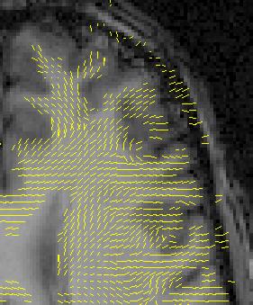
Images representing 2D projections of vectors or tensors may be overlayed on pixel images, yielding compound images. An example is shown in figure Figure 2-2.
The default visualisation for whole images of scalar values is a scaled greyscale map; for overlay images a scaled non-greyscale colour map is the default.
The default visualisation for images of 3-element vector values is the corresponding 2D directional projection in the image plane, after a global scaling, with colour coding indicating the magnitude.
The default visualisation for images of 6-element vector values is the 2D projection of the corresponding ellipsoidal representation in the image plane, after a global scaling, with colour coding indicating the volume.
Geometrical Models
The VM will be able to render 3D geometric objects—meshes, surfaces and volumes—with variable rotation and scale.
Scalar and RGB values associated with volume elements will be displayed through the colour of the enclosing surfaces, in the scalar case using colour maps selectable for each view.
Scalar and RGB values associated with surface elements (polygons) will be displayed through the colour of the surfaces, in the scalar case using colour maps selectable for each view. Colour values associated with a surface override colour values associated with enclosed volumes.
Scalar and RGB values associated with vertices will be displayed through the colour of vertices and, where applicable, edge and surface elements. The colour of the latter will be interpolated between the colours of the vertices defining the surface element, in the scalar case using colour maps selectable for each view. Colour values associated with a vertex override colour values associated with enclosed surfaces or volumes. An example is shown in figure Figure 2-3.

The VM will be capable of scaling scalar data to employ the full range of the chosen colour map.
Scalar values associated with vertices may alternatively be displayed as iso-lines over the surface defined by the vertices.
Scalar representation of multivariate data, such as magnitude of complex number and 3-element vectors and volume of 6-element tensors, will be displayed just like scalar values.
Complex numbers associated with volume elements, surface elements and vertices will be visualised by representing the real and imaginary components by different orthogonal colours (RGB or CMY), specifying the colour of the model surface according to the scheme governing scalar values. This may be combined with intensity indicating the magnitude.
3-element vectors will be displayed directly at the corresponding position (vertex position or surface or volume centre) in the 3D space. They may be directional or undirectional. This may be combined with colour or intensity indicating the magnitude. The vectors may be subjected to a global re-scaling.
6-element tensors will be displayed directly at the corresponding position (see prev. para.) in the 3D space, using a 3D ellipsoidal representations, so called smarties. This may be combined with colour or intensity indicating the volume. The tensors may be subjected to a global re-scaling. An example is shown in figure Figure 2-4.

Anisotropy of tensors associated with volume elements, surface elements and vertices will be visualised by representing the three main cases (isotropic, planar and linear) by different orthogonal colours (RGB or CMY), specifying the colour of the model surface according to the scheme governing scalar values. This may be combined with intensity indicating the volume.
Scalar data (explicit or derived, e.g. magnitude) may be used to define an element mask, such that elements falling out of range may be displayed with a for this purpose specified colour. An example is shown in figure Figure 2-3.
The VM will offer the use of clipping planes for excluding parts of a geometrical dataset from being visualised.
Several geometrical models may be displayed in a single view.
Special Data Objects
Following data objects will be subject to special treatment by the VM:
electrode,
dipole and
streamline.
electrodes, which may have an empty value field, will be plotted in 3D using an electrode glyph; alternatively, they may have a scalar value field, which will be represented by the colour coding of the glyph. The may also have a 3-element normal vector giving the orientation of the glyph.
dipoles will be plotted as 3D vectors, centred at the corresponding vertex position, with a positive and negative pole (half) coloured red and blue, respectively.
streamlines are assumed to consists of a connected set of vertices, possibly with an associated scalar attribute representing the strength of the streamline. The will be visualised as a set of connected `tubes' along the edges connecting the vertices, where the strengths is indicated by the thickness of the tubes.
Generation of Animations
The VM will offer the possibility to generate animations that may be transformed into common animation formats (see the section called Export Formats).
Animations may be generated from data objects with a temporal dimension, where each time step in the data will be shown in one or more frames in the animation, as selected by the user.
Animations maybe generated from a sequence of changes in the viewing parameters, controlling the view of a geometric object. An example would be an animation with a rotating brain.
Other Functional Requirements
In addition to the key functionality defined in the previous sections, the VM will deliver functionality allowing the user to conveniently specify input data for other SimBio routines. It will also offer the possibility to export visualised results in at least one common graphic format.
User Interaction
The user will be able to interactively probe the value (scalar or vector valued) associated with any grid position in a SimBio data set.
The VM will offer the user the possibility to associate vectors representing mechanical forces or electric dipoles, with vertices in a given data set and save these together with the data set. An example is shown in figure Figure 2-5.
The VM will offer the user the possibility to 'tag' vertices in a given data set and save tags these together with the data set. This may for example be used to mark fixed boundary vertices for simulations.

Export Formats
The VM will support export of visualisation results in common graphics and animation formats.
The VM will be to export images in formats employing
lossless or no compression (e.g. PNG, TIFF and PNM), as well as
`lossy' compression (e.g. JPEG).
Several tools exist, freely available on the Internet, for converting between these formats, as well as into other formats. These tools may be distributed together with the SimBio VM.
The VM will not support direct generation of animations. However, it will support batch export of sets of images corresponding to a temporally changing data object, into a set of graphic files in one of previously listed graphic export formats. Again, several freely available tools exist for compiling such sets of graphic files into a single animation.
The SimBio VM will offer an integrated interface to the tool ImageMagick™, if available, for export of visualisation results.